Introduction¶

Overview¶

kALDo is a versatile and scalable open-source software to compute phonon transport in crystalline and amorphous solids. It features real space QHGK calculations and three different solvers of the linearized BTE: direct inversion, self-consistent cycle, and RTA.

The software seamlessly interfaces with popular ab initio codes (Quantum ESPRESSO, VASP), molecular dynamics packages (LAMMPS), and state-of-the-art machine-learned potentials (NEP, MACE, MatterSim, Orb), enabling thermal transport studies from 0 K to finite temperatures.

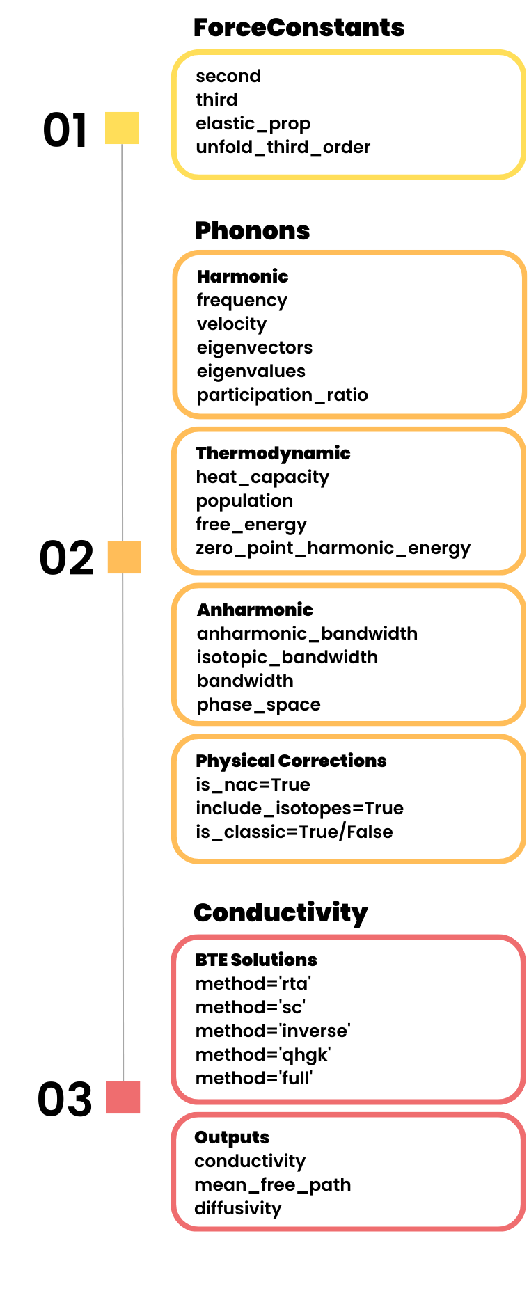
kALDo input/output ecosystem showing integration with diverse force constant sources.

What’s New in 2.0¶

• TDEPSupport: Native integration with temperature-dependent effective potentials for materials with strong anharmonicity

• Machine-Learned Potentials: Seamless integration with NEP, MACE, MatterSim, Orb, and other MLPs via ASE. For benchmarks comparing MLP accuracy, see Matbench Discovery.

• Anharmonicity Diagnostics: σ_A score to quantify anharmonic strength before expensive calculations

• QHA Thermal Expansion: Quasi-harmonic approximation for temperature-dependent lattice properties

• Elastic Properties: Calculate elastic constants from force constants

• Flexible Storage: Multiple backends (formatted, numpy, hdf5, memory) for different use cases

• JSON CLI: Command-line interface for batch processing on HPC systems

Architecture¶

kALDo implements a hierarchical workflow with three core classes:

• ForceConstants: Manages second- and third-order IFCs with methods for importing from external codes or direct calculation via ASE

• Phonons: Computes vibrational properties including frequencies, velocities, scattering rates, heat capacities, and populations

• Conductivity: Solves for thermal transport via BTE (RTA, self-consistent, inverse) or QHGK methods

kALDo class structure showing the three main components and their relationships.

Features¶

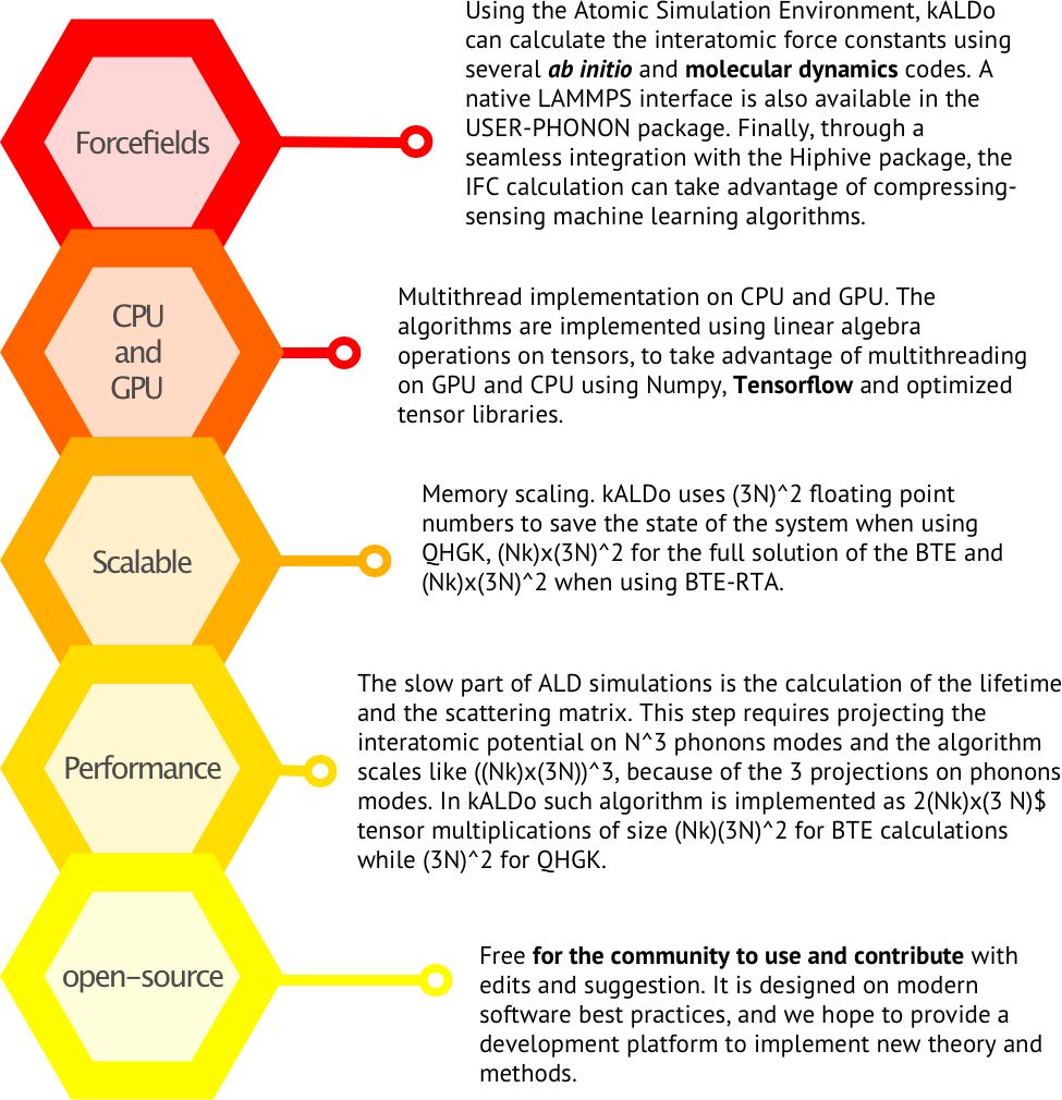
Forcefields. Using the Atomic Simulation Environment (ASE), kALDo can calculate the interatomic force constants using several ab-initio and molecular dynamics codes. A native LAMMPS interface is also available in the USER-PHONON package. Through seamless integration with the HiPhive package, the IFC calculation can take advantage of compressing-sensing machine learning algorithms. Version 2.0 adds native support for modern MLPs including NEP, MACE, MatterSim, and Orb.

CPUs and GPUs. Multithread implementation on CPUs and GPUs. The algorithms are implemented using linear algebra operations on tensors, to take advantage of multithreading on GPU and CPU using Numpy, Tensorflow and optimized tensor libraries.

Scalable. In a system of N atoms and N_k k points, kALDo uses (3N)² floating point numbers to save the state of the system when using QHGK, (N_k × 3N)² for the full solution of the BTE and N_k × 3N² when using BTE-RTA.

Performance. The bottleneck in ALD simulations is the calculation of phonon lifetimes and scattering matrices. This step requires projecting the interatomic potential on 3N phonon modes and scales like (N_k × 3N)³. In kALDo this is implemented as tensor multiplications, with GPU acceleration providing 5-10× speedup for systems with >50 atoms.

Theory¶

Computational Workflow¶

Thermal transport calculations in kALDo proceed through three main stages:

Stage 1: Force Constant Generation. Second and third-order interatomic force constants (IFCs) are computed or imported. These tensors encode harmonic and anharmonic interatomic interactions. Methods include: (i) finite-difference calculations with user-specified atomic displacements, (ii) direct import from density functional perturbation theory (DFPT) calculations, (iii) extraction from molecular dynamics trajectories via TDEP, or (iv) loading from external codes in various file formats.

Stage 2: Phonon Property Computation. The dynamical matrix constructed from second-order IFCs is diagonalized to obtain phonon frequencies, eigenvectors, and group velocities. Third-order IFCs are projected onto phonon eigenstates to compute scattering phase space and rates. Additional properties including heat capacities, populations (Bose-Einstein or classical), and optional isotopic scattering rates are calculated.

Stage 3: Thermal Conductivity Calculation. The BTE or QHGK formalism is employed using phonon properties from Stage 2. Multiple solution methods are available depending on accuracy requirements, memory constraints, and material characteristics.

Interatomic Force Constants¶

Accurate thermal transport predictions require precise determination of interatomic force constants (IFCs), which describe the potential energy surface governing atomic motion. The Taylor expansion of the potential energy \(\phi\) around equilibrium atomic positions in terms of atomic displacements \(u_{i\alpha}\) (atom \(i\), Cartesian direction \(\alpha\)) provides the foundation:

The mass-scaled second-order IFCs define the dynamical matrix:

Phonon frequencies \(\omega_\mu\) and polarization vectors \(\eta_{i\alpha\mu}\) satisfy the eigenvalue equation:

Phonon Properties¶

Group Velocities¶

Phonon group velocity is computed as:

Phonon Populations and Heat Capacity¶

The equilibrium phonon population follows Bose-Einstein statistics:

The modal heat capacity is:

The flag is_classic controls whether quantum or classical statistics are employed.

Three-Phonon Scattering¶

The phonon lifetime from anharmonic scattering is:

Thermal Conductivity Methods¶

Boltzmann Transport Equation¶

The thermal conductivity is:

Three BTE solution methods are implemented:

Quasi-Harmonic Green-Kubo (QHGK)¶

For disordered or amorphous materials where translational symmetry is broken, the QHGK method provides lattice dynamics-based thermal conductivity predictions:

Unlike BTE which treats phonons as plane waves, QHGK naturally captures diffuson and locon contributions in disordered systems.

Physical Modeling Extensions¶

• Isotopic Scattering: Enable via include_isotopes=True

• Non-Analytical Corrections (NAC): For polar materials with LO-TO splitting, enable via is_nac=True

• Finite-Size Effects: Specify sample dimensions via length=(L_x, L_y, L_z) in Angstroms

User Guide¶

Supported Force Constant Formats¶

kALDo supports importing force constants from multiple sources via ForceConstants.from_folder():

Machine-Learned Potentials¶

Example using MatterSim:

from kaldo.forceconstants import ForceConstants
from kaldo.phonons import Phonons
from kaldo.conductivity import Conductivity
from ase.build import bulk
from ase.optimize import BFGS
from ase.constraints import StrainFilter
from mattersim.forcefield import MatterSimCalculator

# Structure optimization
atoms = bulk('SiC', 'zincblende', a=4.35)
calc = MatterSimCalculator(device='cuda')
atoms.calc = calc
sf = StrainFilter(atoms)
opt = BFGS(sf)
opt.run(fmax=0.001)

# Compute force constants
fc = ForceConstants(
    atoms=atoms,
    supercell=[10, 10, 10],
    third_supercell=[5, 5, 5],
    folder='fd_SiC_MatterSim'
)
fc.second.calculate(calc, delta_shift=0.03)
fc.third.calculate(calc, delta_shift=0.03)

# Calculate thermal conductivity
phonons = Phonons(
    forceconstants=fc,
    kpts=[15, 15, 15],
    temperature=300,
    is_classic=False,
    folder='ALD_SiC_MatterSim'
)
cond = Conductivity(phonons=phonons, method='inverse')
print(f"Thermal conductivity: {cond.conductivity.sum(axis=0).trace()/3:.1f} W/m/K")

Storage Backends¶

JSON Command-Line Interface¶

kALDo accepts JSON configuration files for batch processing:

{
  "forceconstants": {
    "folder": "path/to/data",
    "format": "eskm",
    "supercell": [3, 3, 3]
  },
  "phonons": {
    "temperature": 300.0,
    "kpts": [5, 5, 5],
    "is_classic": false
  },
  "conductivity": {
    "method": "rta"
  }
}

Execute with: kaldo < config.json

Units¶