Wurtzite Aluminum Nitride Ace Pyace
Anharmonic Lattice Dynamics (ALD) for \(\ce{w-AlN}\) with ACE
Import Necessary Packages
[1]:
from ase.io import read
from ase.visualize.plot import plot_atoms
import pandas as pd
from pylab import *
import warnings
warnings.filterwarnings("ignore")
Custom Define Functions
[2]:
def cumulative_cond_cal(observables, kappa_tensor, prefactor=1/3):

    """Compute cumulative conductivity based on either frequency or mean-free path

       input:
       observables: (ndarray) either phonon frequency or mean-free path
       cond_tensor: (ndarray) conductivity tensor
       prefactor: (float) prefactor to average kappa tensor, 1/3 for bulk material

       ouput:
       observeables: (ndarray) sorted phonon frequency or mean-free path
       kappa_cond (ndarray) cumulative conductivity

    """

    # Sum over kappa by directions
    kappa = np.einsum('maa->m', prefactor * kappa_tensor)

    # Sort observables
    observables_argsort_indices = np.argsort(observables)
    cumulative_kappa = np.cumsum(kappa[observables_argsort_indices])
    return observables[observables_argsort_indices], cumulative_kappa


def set_fig_properties(ax_list, panel_color_str='black', line_width=2):
    tl = 4
    tw = 2
    tlm = 2

    for ax in ax_list:
        ax.tick_params(which='major', length=tl, width=tw)
        ax.tick_params(which='minor', length=tlm, width=tw)
        ax.tick_params(which='both', axis='both', direction='in',
                       right=True, top=True)
        ax.spines['bottom'].set_color(panel_color_str)
        ax.spines['top'].set_color(panel_color_str)
        ax.spines['left'].set_color(panel_color_str)
        ax.spines['right'].set_color(panel_color_str)

        ax.spines['bottom'].set_linewidth(line_width)
        ax.spines['top'].set_linewidth(line_width)
        ax.spines['left'].set_linewidth(line_width)
        ax.spines['right'].set_linewidth(line_width)

        for t in ax.xaxis.get_ticklines(): t.set_color(panel_color_str)
        for t in ax.yaxis.get_ticklines(): t.set_color(panel_color_str)
        for t in ax.xaxis.get_ticklines(): t.set_linewidth(line_width)
        for t in ax.yaxis.get_ticklines(): t.set_linewidth(line_width)
Denote Latex Font for Plots
[3]:
# Denote plot default format
aw = 2
fs = 12
font = {'size': fs}
matplotlib.rc('font', **font)
matplotlib.rc('axes', linewidth=aw)

# Configure Matplotlib to use a LaTeX-like style without LaTeX
plt.rcParams['text.usetex'] = False
plt.rcParams['font.family'] = 'serif'
plt.rcParams['mathtext.fontset'] = 'cm'
Illustrate Crystal Structure and Elastic Constants
DFT reference for the elastic modulus is adopted from: https://next-gen.materialsproject.org/materials/mp-661
[4]:
# Denote data path
data_folder = "kaldo_runs/"

# Extract supercell structure for later display
atoms = read(data_folder  + 'fd_ACE/replicated_atoms.xyz')

# Retrieve elastic constants and compute bulk modulus
Cijs = np.load(data_folder + 'Cij.npy')
C11 = Cijs[0, 0, 0, 0]
C12 = Cijs[0, 0, 1, 1]
C13 = Cijs[0, 0, 2, 2]
C33 = Cijs[2, 2, 2, 2]
Bulk_modulus = (2*(C11 + C12) + 4*C13 + C33) / 9

# Display supercell and bulk modulus side by side
figure(figsize=(4, 3))
set_fig_properties([gca()])
plot_atoms(atoms)
gca().axis('off')
gca().set_title('w-AlN supercell')
show()

print('\n')

# Prepare data for pandas
df = pd.DataFrame({
    "Properties": ["C11", "C12", "C13", "C33", "Bulk Modulus"],
    "Predictions (GPa)": [C11, C12, C13, C33, Bulk_modulus],
    "DFT references (GPa)": [379, 128, 96, 355, 195]
})

# Format the floats to one decimal place and print
pd.set_option('display.float_format', '{:.1f}'.format)
print(df.to_string(index=False))
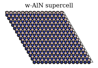
  Properties  Predictions (GPa)  DFT references (GPa)
         C11              367.4                   379
         C12              123.1                   128
         C13              121.6                    96
         C33              345.1                   355
Bulk Modulus              201.4                   195
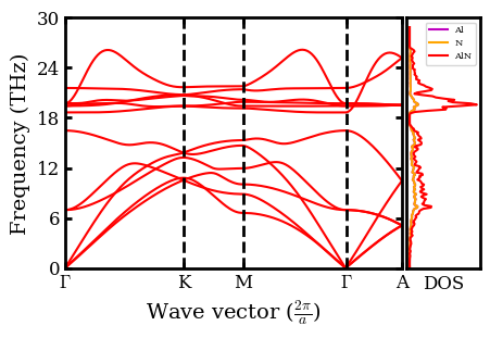
Plot Phonon Spectra (Dispersion) and Density of State (DOS)
[5]:
# Derive symbols for high symmetry directions in Brillouin zone
dispersion = np.loadtxt(data_folder  + 'plots/15_15_9/dispersion')
point_names = np.loadtxt(data_folder  + 'plots/15_15_9/point_names', dtype=str)

point_names_list = []
for point_name in point_names:
    if point_name == 'G':
        point_name = r'$\Gamma$'
    elif point_name == 'U':
        point_name = 'U=K'
    point_names_list.append(point_name)

# Load in the "tick-mark" values for these symbols
q = np.loadtxt(data_folder  + 'plots/15_15_9/q')
Q = np.loadtxt(data_folder  + 'plots/15_15_9/Q_val')

# Load in grid and dos individually
dos_AlN = np.load(data_folder + 'plots/15_15_9/dos.npy')
pdos_Al = np.load(data_folder + 'plots/15_15_9/pdos_Al.npy')
pdos_N = np.load(data_folder + 'plots/15_15_9/pdos_N.npy')

# Plot dispersion
fig = figure(figsize=(4,3))
set_fig_properties([gca()])
plot(q[0], dispersion[0, 0], 'r-', ms=1)
plot(q, dispersion, 'r-', ms=1)
for i in range(1, 4):
    axvline(x=Q[i], ymin=0, ymax=2, ls='--',  lw=2, c="k")
ylabel('Frequency (THz)', fontsize=14)
xlabel(r'Wave vector ($\frac{2\pi}{a}$)', fontsize=14)
gca().set_yticks(np.arange(0, 36, 6))
xticks(Q, point_names_list)
ylim([-0.1, 30])
xlim([Q[0], Q[4]])
dosax = fig.add_axes([0.91, .11, .17, .77])
set_fig_properties([gca()])

# Plot per projection
for p_Al in np.expand_dims(pdos_Al[1],0):
        dosax.plot(p_Al, pdos_N[0], c='m', label='Al')
for p_N in np.expand_dims(pdos_Al[1],0) :
        dosax.plot(p_N, pdos_N[0], c='orange', label='N')
for d in np.expand_dims(dos_AlN[1],0):
    dosax.plot(d, dos_AlN[0],c='r', label='AlN')
dosax.set_yticks([])
dosax.set_xticks([])
dosax.set_xlabel("DOS")
dosax.legend(fontsize=6)
ylim([-0.1, 30])
show()
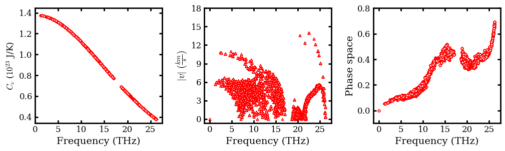
Plot Heat Capacity, Group Velocities and Phase Space
[6]:
# Load in group velocity, heat_capacity (cv) and frequency data
frequency =  np.load(
    data_folder + 'ALD_AlN_ACE/15_15_9/frequency.npy',
    allow_pickle=True)

cv =  np.load(
    data_folder + 'ALD_AlN_ACE/15_15_9/300/quantum/heat_capacity.npy',
    allow_pickle=True)


group_velocity = np.load(
    data_folder + 'ALD_AlN_ACE/15_15_9/velocity.npy')

phase_space = np.load(data_folder +
 'ALD_AlN_ACE/15_15_9/300/quantum/_ps_and_gamma.npy',
                      allow_pickle=True)[:,0]

# Compute norm of group velocity
# Convert the unit from angstrom / picosecond to kilometer/ second
group_velcotiy_norm = np.linalg.norm(
    group_velocity.reshape(-1, 3), axis=1) / 10.0

# Plot observables in subplot
figure(figsize=(12, 3))
subplot(1,3, 1)
set_fig_properties([gca()])
scatter(frequency.flatten(order='C')[3:], 1e23*cv.flatten(order='C')[3:],
        facecolor='w', edgecolor='r', s=10, marker='8')
ylabel (r"$C_{v}$ ($10^{23}$ J/K)")
xlabel('Frequency (THz)', fontsize=14)
ylim(0.9*1e23*cv.flatten(order='C')[3:].min(), 1.05*1e23*cv.flatten(order='C')[3:].max())
gca().set_xticks(np.arange(0, 30, 5))

subplot(1 ,3, 2)
set_fig_properties([gca()])
scatter(frequency.flatten(order='C'),
        group_velcotiy_norm, facecolor='w', edgecolor='r', s=10, marker='^')
xlabel('Frequency (THz)', fontsize=14)
ylabel(r'$|v| \ (\frac{km}{s})$', fontsize=14)
gca().set_xticks(np.arange(0, 30, 5))
gca().set_yticks(np.arange(0, 21, 3))

subplot(1 ,3, 3)
set_fig_properties([gca()])
scatter(frequency.flatten(order='C'),
        phase_space, facecolor='w', edgecolor='r', s=10, marker='o')
ylim([-0.1, 0.8])
gca().set_xticks(np.arange(0, 30, 5))
xlabel('Frequency (THz)', fontsize=14)
ylabel('Phase space', fontsize=14)
subplots_adjust(wspace=0.33)
show()
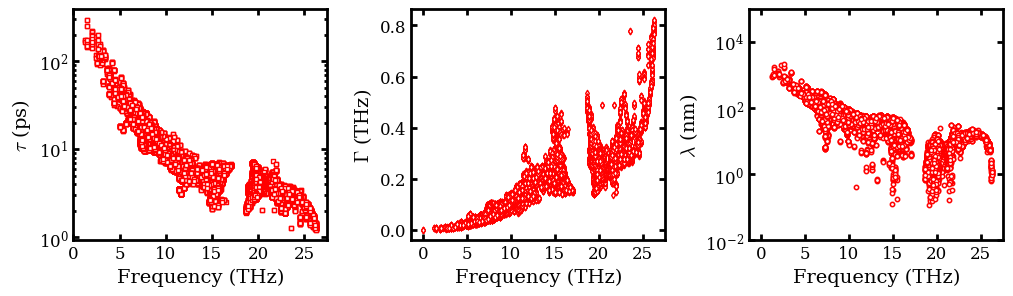
Plot Phonon Lifetime (\(\tau\)), Scattering Rate (\(\Gamma\)) \(\&\) MFP (\(\lambda\))
Note that \(\Gamma\) and \(\tau\) are computed only with the relaxation time approximation (RTA).
[7]:
# Load in scattering rate
scattering_rate = np.load(
    data_folder +
    'ALD_AlN_ACE/15_15_9/300/quantum/bandwidth.npy', allow_pickle=True)

# Derive lifetime, which is inverse of scattering rate
life_time = scattering_rate ** (-1)

# Denote lists to intake mean free path in each direction
mean_free_path = []
for i in range(3):
    mean_free_path.append(np.loadtxt(
    data_folder +
    'ALD_AlN_ACE/15_15_9/inverse/300/quantum/mean_free_path_' +
    str(i) + '.dat'))

# Convert list to numpy array and compute norm for mean free path
# Convert the unit from angstrom  to nanometer
mean_free_path = np.array(mean_free_path).T
mean_free_path_norm = np.linalg.norm(
    mean_free_path.reshape(-1, 3), axis=1) / 10.0

# Plot observables in subplot
figure(figsize=(12, 3))
subplot(1,3, 1)
set_fig_properties([gca()])
scatter(frequency.flatten(order='C'),
        life_time, facecolor='w', edgecolor='r', s=10, marker='s')
yscale('log')
ylabel(r'$\tau$ (ps)', fontsize=14)
xlabel('Frequency (THz)', fontsize=14)
gca().set_xticks(np.arange(0, 30, 5))

subplot(1,3, 2)
set_fig_properties([gca()])
scatter(frequency.flatten(order='C'),
        scattering_rate, facecolor='w', edgecolor='r', s=10, marker='d')
ylabel(r'$\Gamma$ (THz)', fontsize=14)
xlabel('Frequency (THz)', fontsize=14)
gca().set_xticks(np.arange(0, 30, 5))

subplot(1,3, 3)
set_fig_properties([gca()])
scatter(frequency.flatten(order='C'),
        mean_free_path_norm, facecolor='w', edgecolor='r', s=10, marker='8')
ylabel(r'$\lambda$ (nm)', fontsize=14)
xlabel('Frequency (THz)', fontsize=14)
yscale('log')
gca().set_xticks(np.arange(0, 30, 5))
ylim([1e-2, 1e5])
subplots_adjust(wspace=0.33)
show()
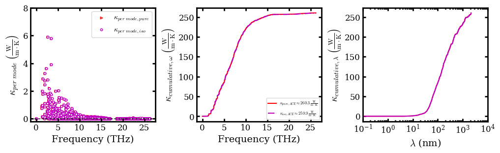
Plot per mode and cumulative \(\kappa\)
[8]:
# Denote zeros to intake kappa tensor
kappa_tensor = np.zeros([mean_free_path.shape[0], 3, 3])
kappa_tensor_iso = np.zeros([mean_free_path.shape[0], 3, 3])

for i in range(3):
    for j in range(3):
        kappa_tensor[:, i, j] = np.loadtxt(data_folder +
    'ALD_AlN_ACE/15_15_9/inverse/300/quantum/conductivity_' +
    str(i) + '_' + str(j) + '.dat')
        kappa_tensor_iso[:, i, j] = np.loadtxt(data_folder +
    'ALD_AlN_ACE/15_15_9/inverse/300/quantum/isotopes/conductivity_' +
    str(i) + '_' + str(j) + '.dat')

# Sum over the 0th dimension to recover 3-by-3 kappa matrix
kappa_matrix = kappa_tensor.sum(axis=0)
print("Bulk thermal conductivity: %.1f W m^-1 K^-1\n"
      %np.mean(np.diag(kappa_matrix)))
print("kappa matrix: ")
print(kappa_matrix)
print('\n')

kappa_matrix_iso = kappa_tensor_iso.sum(axis=0)
print("Bulk thermal conductivity with isotopic scattering: %.1f W m^-1 K^-1\n"
      %np.mean(np.diag(kappa_matrix_iso)))
print("kappa matrix with isotopic scattering: ")
print(kappa_matrix_iso)
print('\n')

# Compute kappa in per mode and cumulative representations
kappa_per_mode = kappa_tensor.sum(axis=-1).sum(axis=1)
freq_sorted, kappa_cum_wrt_freq = cumulative_cond_cal(
    frequency.flatten(order='C'), kappa_tensor)
lambda_sorted, kappa_cum_wrt_lambda = cumulative_cond_cal(
    mean_free_path_norm, kappa_tensor)

kappa_per_mode_iso = kappa_tensor_iso.sum(axis=-1).sum(axis=1)
freq_sorted, kappa_cum_wrt_freq_iso = cumulative_cond_cal(
    frequency.flatten(order='C'), kappa_tensor_iso)
lambda_sorted, kappa_cum_wrt_lambda_iso = cumulative_cond_cal(
    mean_free_path_norm, kappa_tensor_iso)

# Plot observables in subplot
figure(figsize=(12, 3))
subplot(1,3, 1)
set_fig_properties([gca()])
scatter(frequency.flatten(order='C'),
        kappa_per_mode, facecolor='w', edgecolor='r', s=10, marker='>', label='$\kappa_{per \ mode, pure }$')
scatter(frequency.flatten(order='C'),
        kappa_per_mode_iso, facecolor='w', edgecolor='m', s=10, marker='o', label='$\kappa_{per \ mode, iso }$')
gca().axhline(y = 0, color='k', ls='--', lw=1)
ylabel(r'$\kappa_{per \ mode}\;\left(\frac{\rm{W}}{\rm{m}\cdot\rm{K}}\right)$',fontsize=14)
xlabel('Frequency (THz)', fontsize=14)
legend(loc=1, fontsize=10)
gca().set_xticks(np.arange(0, 30, 5))
ylim([-0.2, 8])

subplot(1,3, 2)
set_fig_properties([gca()])
plot(freq_sorted, kappa_cum_wrt_freq, 'r',
     label=r'$\kappa_{pure, ACE} \approx 260.3\;\frac{\rm{W}}{\rm{m}\cdot\rm{K}}$')
plot(freq_sorted, kappa_cum_wrt_freq_iso, c='m',
     ls='-.', label=r"$\kappa_{iso, ACE} \approx 259.9\;\frac{\rm{W}}{\rm{m}\cdot\rm{K}}$")
gca().set_yticks(np.arange(0, 300, 50))
ylabel(r'$\kappa_{cumulative, \omega}\;\left(\frac{\rm{W}}{\rm{m}\cdot\rm{K}}\right)$',fontsize=14)
xlabel('Frequency (THz)', fontsize=14)
gca().set_xticks(np.arange(0, 30, 5))
legend(loc=4, fontsize=6)

subplot(1,3, 3)
set_fig_properties([gca()])
plot(lambda_sorted, kappa_cum_wrt_lambda, 'r')
plot(lambda_sorted, kappa_cum_wrt_lambda_iso, c='m')
gca().set_yticks(np.arange(0, 300, 50))
xlabel(r'$\lambda$ (nm)', fontsize=14)
ylabel(r'$\kappa_{cumulative, \lambda}\;\left(\frac{\rm{W}}{\rm{m}\cdot\rm{K}}\right)$',fontsize=14)
xscale('log')
xlim([1e-1, 1e4])
subplots_adjust(wspace=0.33)
show()
Bulk thermal conductivity: 260.3 W m^-1 K^-1

kappa matrix:
[[ 2.64608547e+02  5.78997217e-01  2.43088665e-01]
 [ 4.18946787e-01  2.64671284e+02 -2.31451194e-01]
 [ 3.69859965e-01  3.98814383e-01  2.51516013e+02]]


Bulk thermal conductivity with isotopic scattering: 259.9 W m^-1 K^-1

kappa matrix with isotopic scattering:
[[ 2.64186375e+02  5.76801222e-01  2.42219797e-01]
 [ 4.17874653e-01  2.64246959e+02 -2.31684048e-01]
 [ 3.66651347e-01  3.93057933e-01  2.51164394e+02]]